Tutorial: Ensemble of DeepProg model

Secondly, we will build a more complex DeepProg model constituted of an ensemble of sub-models, each originated from a subset of the data. For that purpose, we need to use the SimDeepBoosting class:

from simdeep.simdeep_boosting import SimDeepBoosting

help(SimDeepBoosting)

Similarly, to the SimDeep class, we define our training dataset

# Location of the input matrices and survival file
from simdeep.config import PATH_DATA

from collections import OrderedDict

# Example tsv files
tsv_files = OrderedDict([
          ('MIR', 'mir_dummy.tsv'),
          ('METH', 'meth_dummy.tsv'),
          ('RNA', 'rna_dummy.tsv'),
])

# File with survival event
survival_tsv = 'survival_dummy.tsv'

Instanciation

Then, we define arguments specific to DeepProg and instanciate an instance of the class

project_name = 'stacked_TestProject'
epochs = 10 # Autoencoder epochs. Other hyperparameters can be fine-tuned. See the example files
seed = 3 # random seed used for reproducibility
nb_it = 5 # This is the number of models to be fitted using only a subset of the training data
nb_threads = 2 # These treads define the number of threads to be used to compute survival function
PATH_RESULTS = "./"

boosting = SimDeepBoosting(
    nb_threads=nb_threads,
    nb_it=nb_it,
    split_n_fold=3,
    survival_tsv=survival_tsv,
    training_tsv=tsv_files,
    path_data=PATH_DATA,
    project_name=project_name,
    path_results=PATH_RESULTS,
    epochs=epochs,
    seed=seed)

Here, we define a DeepProg model that will create 5 SimDeep instances each based on a subset of the original training dataset.the number of instance is defined by he nb_it argument. Other arguments related to the autoencoders construction can be defined during the class instanciation, such as epochs.

Fitting

Once the model is defined we can fit it

# Fit the model
boosting.fit()
# Predict and write the labels
boosting.predict_labels_on_full_dataset()

Some output files are generated in the output folder:

stacked_TestProject
├── stacked_TestProject_full_labels.tsv
├── stacked_TestProject_KM_plot_boosting_full.png
├── stacked_TestProject_proba_KM_plot_boosting_full.png
├── stacked_TestProject_test_fold_labels.tsv
└── stacked_TestProject_training_set_labels.tsv

The inferred labels, labels probability, survival time, and event are written in the stacked_TestProject_full_labels.tsv file:

sample_test_48  1       0.474781026865  332.0   1.0
sample_test_49  1       0.142554926379  120.0   0.0
sample_test_46  1       0.355333486034  355.0   1.0
sample_test_47  0       0.618825352398  48.0    1.0
sample_test_44  1       0.346797097671  179.0   0.0
sample_test_45  1       0.0254692404734 360.0   0.0
sample_test_42  1       0.441997226254  346.0   1.0
sample_test_43  1       0.0783603292911 335.0   0.0
sample_test_40  1       0.380182410315  149.0   0.0
sample_test_41  0       0.953659261728  155.0   1.0

Note that the label probablity corresponds to the probability to belongs to the subtype with the lowest survival rate. Two KM plots are also generated, one using the cluster labels:

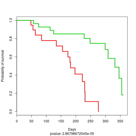KM plot 3

and one using the cluster label probability dichotomized:

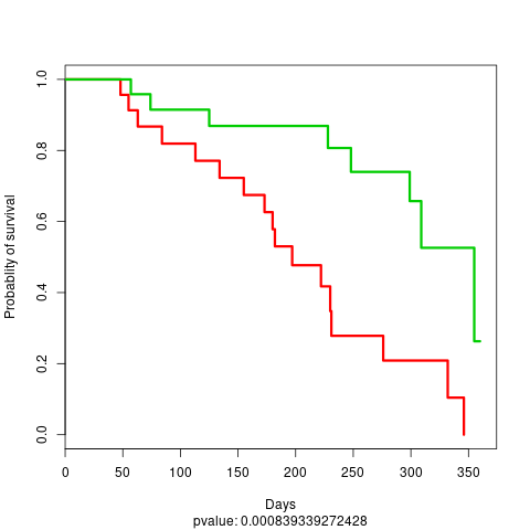KM plot 4

We can also compute the feature importance per cluster:

# oOmpute the feature importance
boosting.compute_feature_scores_per_cluster()
# Write the feature importance
boosting.write_feature_score_per_cluster()

The results are updated in the output folder:

stacked_TestProject
├── stacked_TestProject_features_anticorrelated_scores_per_clusters.tsv
├── stacked_TestProject_features_scores_per_clusters.tsv
├── stacked_TestProject_full_labels.tsv
├── stacked_TestProject_KM_plot_boosting_full.png
├── stacked_TestProject_proba_KM_plot_boosting_full.png
├── stacked_TestProject_test_fold_labels.tsv
└── stacked_TestProject_training_set_labels.tsv

Evaluate the models

DeepProg allows to compute specific metrics relative to the ensemble of models:

# Compute internal metrics
boosting.compute_clusters_consistency_for_full_labels()

# Collect c-index
boosting.compute_c_indexes_for_full_dataset()
# Evaluate cluster performance
boosting.evalutate_cluster_performance()
# Collect more c-indexes
boosting.collect_cindex_for_test_fold()
boosting.collect_cindex_for_full_dataset()
boosting.collect_cindex_for_training_dataset()

# See Ave. number of significant features per omic across OMIC models
boosting.collect_number_of_features_per_omic()

Predicting on test dataset

We can then load and evaluate a first test dataset

boosting.load_new_test_dataset(
    {'RNA': 'rna_dummy.tsv'}, # OMIC file of the test set. It doesnt have to be the same as for training
    'TEST_DATA_1', # Name of the test test to be used
    'survival_dummy.tsv', # [OPTIONAL] Survival file of the test set. USeful to compute accuracy metrics on the test dataset
)

# Predict the labels on the test dataset
boosting.predict_labels_on_test_dataset()
# Compute C-index
boosting.compute_c_indexes_for_test_dataset()
# See cluster consistency
boosting.compute_clusters_consistency_for_test_labels()

We can load an evaluate a second test dataset

boosting.load_new_test_dataset(
    {'MIR': 'mir_dummy.tsv'}, # OMIC file of the test set. It doesnt have to be the same as for training
    'TEST_DATA_2', # Name of the test test to be used
    'survival_dummy.tsv', # Survival file of the test set
)

# Predict the labels on the test dataset
boosting.predict_labels_on_test_dataset()
# Compute C-index
boosting.compute_c_indexes_for_test_dataset()
# See cluster consistency
boosting.compute_clusters_consistency_for_test_labels()

The output folder is updated with the new output files

stacked_TestProject
├── stacked_TestProject_features_anticorrelated_scores_per_clusters.tsv
├── stacked_TestProject_features_scores_per_clusters.tsv
├── stacked_TestProject_full_labels.tsv
├── stacked_TestProject_KM_plot_boosting_full.png
├── stacked_TestProject_proba_KM_plot_boosting_full.png
├── stacked_TestProject_TEST_DATA_1_KM_plot_boosting_test.png
├── stacked_TestProject_TEST_DATA_1_proba_KM_plot_boosting_test.png
├── stacked_TestProject_TEST_DATA_1_test_labels.tsv
├── stacked_TestProject_TEST_DATA_2_KM_plot_boosting_test.png
├── stacked_TestProject_TEST_DATA_2_proba_KM_plot_boosting_test.png
├── stacked_TestProject_TEST_DATA_2_test_labels.tsv
├── stacked_TestProject_test_fold_labels.tsv
├── stacked_TestProject_test_labels.tsv
└── stacked_TestProject_training_set_labels.tsv

file: stacked_TestProject_TEST_DATA_1_KM_plot_boosting_test.png

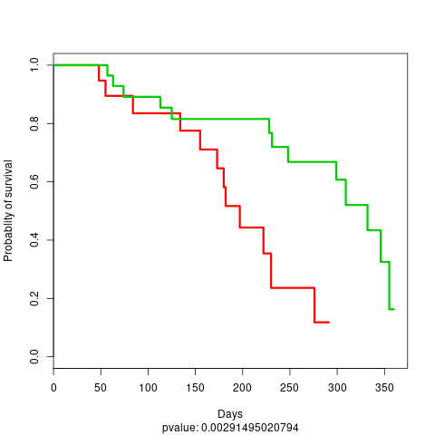test KM plot 1

file: stacked_TestProject_TEST_DATA_2_KM_plot_boosting_test.png

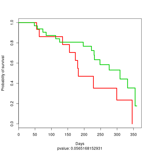test KM plot 2

Distributed computation

Because SimDeepBoosting constructs an ensemble of models, it is well suited to distribute the individual construction of each SimDeep instance. To do such a task, we implemented the use of the ray framework that allow DeepProg to distribute the creation of each submodel on different clusters/nodes/CPUs. The configuration of the nodes / clusters, or local CPUs to be used needs to be done when instanciating a new ray object with the ray API. It is however quite straightforward to define the number of instances launched on a local machine such as in the example below in which 3 instances are used.

# Instanciate a ray object that will create multiple workers
import ray
ray.init(webui_host='0.0.0.0', num_cpus=3)
# More options can be used (e.g. remote clusters, AWS, memory,...etc...)
# ray can be used locally to maximize the use of CPUs on the local machine
# See ray API: https://ray.readthedocs.io/en/latest/index.html

boosting = SimDeepBoosting(
    ...
    distribute=True, # Additional option to use ray cluster scheduler
    ...
)
...
# Processing
...

# Close clusters and free memory
ray.shutdown()

More examples

More example scripts are availables in ./examples/ which will assist you to build a model from scratch with test and real data:

examples
├── create_autoencoder_from_scratch.py # Construct a simple deeprog model on the dummy example dataset
├── example_with_dummy_data_distributed.py # Process the dummy example dataset using ray
├── example_with_dummy_data.py # Process the dummy example dataset
└── load_3_omics_model.py # Process the example HCC dataset